Villin Headpiece

To provide examples of ID applications, we used trajectories of fast folding proteins generated by D. E. Shaw group (DOI:10.1126/science.1208351).

In particular, we used chicken villin headpiece (PDB: 2F4K), a 35 residue long protein with two point mutations, K65(NLE) and K70(NLE), to increase the folding speed up to 5 times in respect to wild-type.

We used protein structure and trajectory data of DESRES-Trajectory_2F4K-0-protein. We sampled the originally simulated trajectory in 6 shorter sub-trajectories of 2000 frames each, representing either the folded state of the protein (f0, f1, f2) or the unfolded one (u0, u1, u2).

Original Trajectory	New Trajectory	Frames	State
2f4k-0-protein-000.dcd	2f4k_u0.xtc	[0:2000]	Unfolded
2f4k-0-protein-001.dcd	2f4k_f0.xtc	[0:2000]	Folded
2f4k-0-protein-001.dcd	2f4k_u1.xtc	[5000:7000]	Unfolded
2f4k-0-protein-004.dcd	2f4k_f1.xtc	[8000:]	Folded
2f4k-0-protein-005.dcd	2f4k_u2.xtc	[1700:3700]	Unfolded
2f4k-0-protein-005.dcd	2f4k_f2.xtc	[5000:7000]	Folded

intrinsic_dimension()

By computing ID as local it is possible to see how this value evolves along the trajectory, we called it Instantaneous ID.

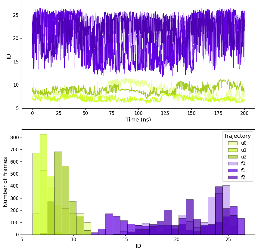
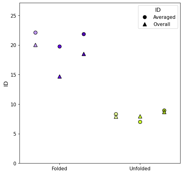
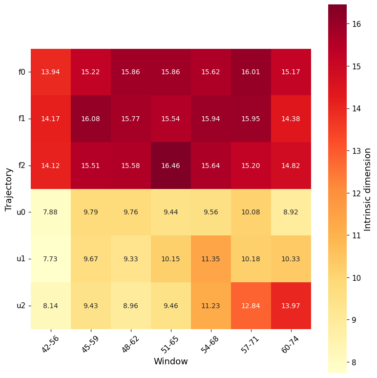
The trajectories are clearly split in two ID groups, so we can divide the trajectories in "folded" and "unfolded" by setting a threshold at ID<13, this shows the capability of ID to identify the two distinct states.

This can be done both with local (including standard deviations) ID and the mean of the global ID along the trajectory.

section_id()

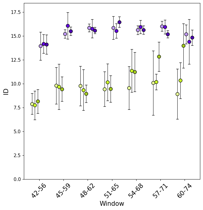
Similarly, with section_id, it is possible to visualise, for each window, the value of ID along the trajectory (both as global ID and local).

In this case it is intresting to notice how some of the windows show a clearer separation between folded and unfolded states than others, for example window 42-56 compared to window 51-56.

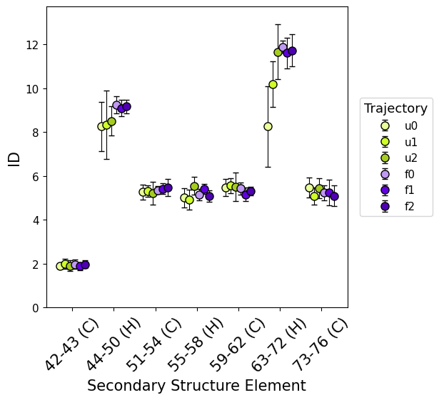
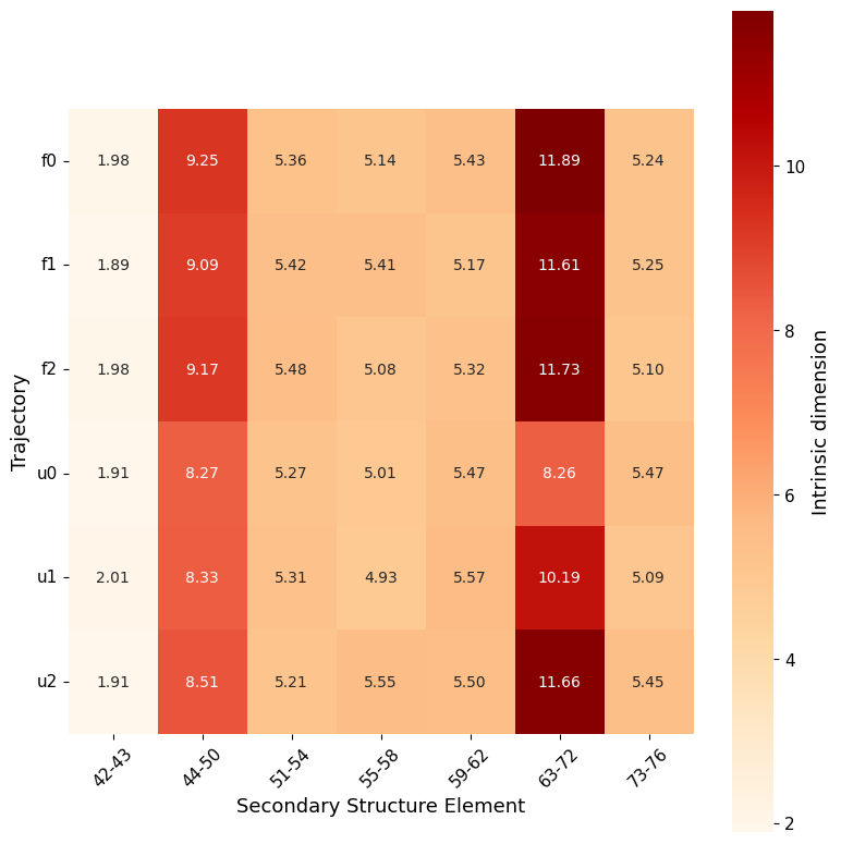
secondary_structure_id()

secondary_structure_id, divides the protein by secondary structure elements instead of same-length windows, estimating ID along the trajectory on each element individually (both as global ID and local).

Computing ID separately for each secondary structure element provides more detailed insights into the protein’s flexibility, as different types of secondary structures comprise distinct levels of flexibility in specific regions.